1. INTRODUCTION
One of the most widely discussed aspects regarding the English Agricultural
Revolution has been quantifying the magnitude of the agricultural product and
GDP per capita. The Agrarian Reform (1536) and Social Revolutions (1640 and
1688) disrupted one of the most useful sources used as a proxy for crop
production in continental Europe in pre-capitalist times: tithes (Kain & Prince, 2006). This lack of data has led to estimations being made from
indirect methods and other sources. From a demand-side approach, agricultural
production has been calculated on the basis of consumption per head,
population, prices and elasticities. From a supply-side approach, on the other
hand, the sources have been a growing set of non-randomly selected
site-specific probate inventories and farm accounts. This methodological
diversity has produced widely varying estimates due to the differing temporal
and spatial features and sources used in each case. For instance, Morgan Kelly
and Cormac Ó Gráda (2013) have called for an upward adjustment of the recent agricultural
production estimated by Stephen Broadberry, Alexander Klein, Mark Overton and
Bas van Leeuwen (2015). There is also an ongoing debate over the dating of the
English Agricultural Revolution, raised by Mark Overton (1996a) and Robert C.
Allen (1991, 2008, 2009). Another open question is whether waves in
agricultural output and productivity might have been responsible for the slow
progress of English economic growth between 1760 and 1815, and for its later
acceleration. To help determine the answers to these questions, Robert Allen
has called for new methods to be developed that allow a better inference of
changes in production and yields (Allen, 1999: 209-211).
In partial response to Allen’s request, the aim of this paper is to estimate an annual series of wheat output
in England between 1645 and 1761. A new method is presented based on Davenant’s Law (1699). Charles Davenant was a contemporary author from that intriguing
period and the first to propose estimating the inverse variations of wheat
harvests from the variations of their prices. He did this using data previously
collected by Gregory King. The usefulness and accuracy of this method has been
highlighted by historians such as Edward Anthony Wrigley (1987) and economists
such as Anthony M. Endres (1987) and Jean-Pascal Simonin (1996). The method is
also currently being used to estimate production from prices when facing
unreliable statistical output data (Nielsen, Smith & Guillén, 2012). We will use it for the same purpose, adding other assumptions, i.e. to estimate a final aggregate gross and net production of wheat –meaning gross output minus seeds, animal feeding and losses– from a demand-side approach, to then compare the outcome with the supply data
assembled by other historians who have considered yields, population growth and
long-term income growth.
Notwithstanding the importance of wheat it is worth stressing other grains, such
as barley, rye and oats, as well as pulses, turnips and clover, potatoes and
livestock. However, as Robert Allen stated, during the transition from
subsistence to market agriculture and urban development wheat dominates the history of crop yields, and the history of wheat shows the
importance of the pre-1750 agricultural revolution (Allen, 1999: 225).
This paper is structured as follows. The first section summarizes the current
debates in agricultural historiography. The second explains the methodology
used to build the new series. The third assesses the results obtained comparing
them with current estimates, and justifies their accuracy. And the fourth
concludes.
2. THE PROBLEM WITH ASSESSING THE ECONOMIC PERFORMANCE OF ENGLISH AGRICULTURE
PRIOR TO 1884
There are no statistical data on the annual physical wheat production in Britain
prior to 1884 (Mitchell, 1988). Neither can we count on any proxy such as
tithes, traditionally used as sources in continental Europe. Thus, over the
last thirty years economic and agricultural historians have had to use other
indicators to assess the performance of English agriculture: total physical
output, yields, agricultural production, consumption and elasticities. As can
be seen in Table 1, physical output estimates are scarce and never annual. One
of the earliest was contributed by Phyllis Deane and W. A. Cole (1967: 62-8)
and showed a rise in wheat production during the 18th century from 29 to 50 million bushels (73%), substantially larger than the
growth in other grains (43%). Gross production can be calculated using the
acreage estimates and Allen’s yields (2005: 28, 32) put forward for the period 1300 to 1850, and this
highlights a dramatic increase in production between 1800 and 1850.
Based on some assumptions regarding the consumption of bread and flour by
labourers, Robert Allen also presented an estimate to support his idea that the
volume of wheat demand was bigger than that put forward by Gregory Clark
(2007), according to which wheat demand would have gradually risen from 40
million bushels in 1770 to 170 or more in 1850, with a rapid increase from 1820
onwards. Allen multiplies the share of bread and flour in the average wages by
the employed population (manual labour). He obtains the total income spent on
bread and flour, which he divides by their respective prices, deducting their
volume. Applying a 2:1 relationship between bread and flour, he calculates the
total wheat demanded in bushels. To do this, he supposes an income elasticity
of bread and flour demand equal to zero at the upper average income levels of
manual labourers. The latest estimates have been presented in Broadberry et al. (2015), with decennial averages of net physical output and cultivated area
taken from a Manorial Accounts Database, a Probate Inventories Database and a
Modern Farm Accounts Database following a supply-side approach. All of these
estimates are summarized in Table 1.
Table 1
Physical output and demand of wheat in millions of bushels, according to different authors, 1650-1884
| Years | Estimate | Type of estimate | Author |
| 1650-59 | 27.01 | Net output | Broadberry et al. (2015) |
| 1700-09 | 27.94 | Net output | Broadberry et al. (2015) |
| 1700 | 30.00 | Gross output | Deane and Cole (1967) |
| 1700 | 26.60 | Gross output | Allen (2005) |
| 1750-59 | 31.48 | Net output | Broadberry et al. (2015) |
| 1750 | 42.00 | Gross output | Allen (2005) |
| 1770 | 40.00 | Demand | Allen (2007) |
| 1800-09 | 46.32 | Net output | Broadberry et al. (2015) |
| 1800 | 50.00 | Gross output | Deane and Cole (1967) |
| 1800 | 50.00 | Demand | Allen (2005) |
| 1850-59 | 73.69 | Net output | Broadberry et al. (2015) |
| 1850 | 100.80 | Gross output | Allen (2005) |
| 1850 | 170.00 | Demand | Allen (2007) |
| 1860-69 | 86.07 | Net output | Broadberry et al.(2015) |
| 1884 | 80.20 | Gross output | British Statistics (1988) |
Source: our own calculation. Calculation from the references given in the table.
A second and much more frequent approach is that related to land productivity
(yields), measured in bushels per acre. Although we can find abundant
information on the Middle Ages, and again in the 19th century, estimates on the early modern era are scarce. This has led researchers
to use intermediate methods, with estimates being elaborated from site-specific
primary sources, mainly local probate inventories (Overton, 1979, 1991, 1996a,
1996b; Allen, 1988, 1989, 1991, 1999; Glennie, 1991; Turner, 1982, 1986;
Theobald, 2002; Yelling, 1970, 1973) and farm accounts (Turner, Becket & Afton, 2001). For the second half of the 18th century and the beginning of the 19th century, there is the well-known work by Arthur Young (see John, 1986). There
are also some public statistics, such as the Harvest Inquiries of 1794, 1795
and 1800, Crop Returns in 1801 (Turner, 1982), and the Board of Agriculture
Surveys in 1816 (see John, 1986). The works of James Caird in 1852, Mark Lane
Express in 1860 and 1861 (John, 1986), or those by John B. Lawes and Joseph H.
Gilbert (1893) regarding the results of the Rothampsted experiments between
1852 and 1884. A summary of all these contributions can be found in a chapter
on the wheat question published by Turner, Beckett and Afton (2001: 116-49).
The figures proposed by M. J. R. Healy and Eric L. Jones (1962) are also
available, based on market studies of Liverpool grain merchants, and from data
published by B. A. Holderness (1989), which reported 16 Net bu/acre in 1750,
19.5 in 1800, 20.5 in 1810, and 26 in 1850.
Liam Brunt (2004, 2015) used another different approach from the supply-side
perspective. This author analysed the production of wheat and its yields. To
control for variability, he used climatic variables (temperatures and
rainfall), which he related to output data registered by the cereal traders of
Liverpool between 1815 and 1859 by means of a regression model (Healy & Jones, 1962). He then predicted crop movements backwards before introducing
technological variables to establish the trend.
All of these data have created a difficult puzzle to fit together. Some basic
facts do seem quite clear, however. Agricultural output per head increased
between 1700 and 1760 (Crafts, 1980). Yet, there is a long debate on what
happened before 1700 and after 1760. Mark Overton (1996a) argued that it was
between 1750 and 1850 that the Agricultural Revolution took place, whereas
Allen pointed out that output grew slowly, and yields fell during the second
half of the 18th century. The first wave of innovations (clover, turnips, new Leicester sheep,
convertible husbandry) did not seem to contribute much to economic growth from
1760 onwards, and Nicholas Crafts even talked about a Malthusian shadow threatening England at the end of the 18th century (Crafts, 1980). It was not until the first half of the 19th century that agricultural output started to rise significantly. Assuming this
would help to explain the slow advance of the first stage of the Industrial
Revolution and the faster next stage. Allen also suggested a three-stage
general chronology: from 1520 to 1739, from 1740 to 1800, and from 1800
onwards. During the first stage, there would have been significant agricultural
growth, also pointed out by Jones (1965) and Kerridge (1967) and other authors.
During the second stage, output only increased 10% (and yields also began to
decline), whereas from 1800 to 1850, agricultural production grew by 65%
(Allen, 1999: 210-25).
According to Gregory Clark (2002: 16-25), population growth during the
Industrial Revolution was largely supported by food imports. Rather than a
productive revolution, there would have been a reorientation of agriculture
towards human feeding. Before 1869, improvements in land yields would have been
much more relevant than in labour productivity. In this author’s opinion, it was a long period of modest but constant advance in crop yields
(1600-1750). After that period, a 50-year pause would have followed, when both
yields and labour productivity decreased. And then, after 1800, land and labour
productivities would start to grow slowly but steadily.
Finally, under another perspective related to consumption, food demand and
elasticities, E. J. T. Collins (1975) claimed that it was not until at least
1745 that the increase of income made wheat the most consumed cereal by the
English population. During the 17th and 18th centuries rye bread, and that made by mixing other cereals, were basic foods. Maslin (wheat and rye bread) and muncorn (barley and oat bread) predominated in the Lowlands. Barley, rye, oat, beans and
pulses marked the prevailing consumption pattern. High substitution elasticity
would explain why England avoided famine (Appleby, 1979; Hoyle, 2013). Even
during the Tudor period, and that of the first Stuarts, Malthusian pressure
reduced wheat consumption. Something similar was claimed by chroniclers of the
time. Gregory King described wheat consumption as being in the minority at the
end of the 17th century. According to Tooke and Newmarch (1838), the increase of wheat bread
consumption was slow. In south-west England, the working classes (including
agricultural labourers and small farmers) consumed barley. In 1795 less than
45% ate wheat bread, while barley still prevailed in the peninsular counties
(55%). In Wales, staple food consisted of barley and oats, whereas in the
Midlands the consumption pattern was more diversified (Collins, 1975: 98-9).
Christian Petersen (1995) dated the beginning of the golden age of wheat bread between 1770 and 1870, not earlier. We know that between 1656
and 1704 wheat became more expensive than rye (its relative price increasing
from 1.23 to 1.89). Although wheat prices decreased later, it was still more
expensive than rye in 1739 (1.43), and from 1750 onwards its exchange rate
worsened again according to our own calculation using Gregory Clark’s prices (2004, 2005, 2007). Using the output estimates of Broadberry et al. (2015: 98, 112), we find that in 1650 wheat would have constituted 38.4% of
grains (27.01 million of bushels on average), and 36.7% in 1750 (31.48 million
bushels on average).
Another sign of increased wheat demand is international trade. It was not until
the 1760s that Great Britain became a wheat importer (Ormrod, 1985). Government
policies must also have had an influence on this fact: several regulations (Assize of Wheat, Bounty Acts) kept wheat prices high thereby affecting domestic consumption (even though it
was decreasing in the long run), a fact harshly criticized by Adam Smith in his
Wealth of Nations (1776). From the second half of the 17th century, export subsidies began to be applied, such as those implemented in
1663 and 1689, although they do seem to have been more effective in the first
half of the 18th century. They were cancelled in periods of scarcity, as in the late nineties of
the 17th century (Comber, 1808; Hipkin, 2012). Some econometric studies also confirm the
influence of Corn Bounties on wheat supply (Tello et al., 2017). At the same time, however, it seems that wheat was the most integrated
cereal in the different English counties as early as the 1690s (Chartres, 1985,
1995) –although this remains a controversial issue.
In summary, it would seem that cereal consumption was diverse in Britain during
the 18th century and wheat did not start to stand out until at least after 1760.
Consequently, it is acceptable to assume that the slow income per head rise was
not initially a significant factor in wheat demand. Whereas farm management in
relation to soil fertility, land yields and labour productivity, together with
weather impacts and expectations, determined the evolution of supply,
population growth was the main driver of wheat demand. This fact suggests an
inverted U-shaped wheat income elasticity (εi) over time. In a first phase, it would be null or very low. As wheat bread –and other wheat products– increasingly started to be consumed and replaced other types of bread to become
a basic product, εi increased. It only fell again when the standards of living improved,
consumption diversified, people’s preferences changed, and basic needs were better met at the end of the 19th century. We know that elasticities are not fixed over time. As recent research
shows, while εi is currently low in both countries where wheat is secondary and well-developed
countries, it is high in under-developed ones (Abler, 2010).
It has also been observed that price elasticity tends to fall when income
elasticity does (Abler, 2010: 21). This trend has been confirmed by Campbell
and Ó Gráda’s work (2011), which showed that the price elasticity of wheat demand fell in
the very long term. These authors analysed Robert Fogel’s (2004) and Gunnar Persson’s (1999) divergent positions on the issue. Fogel assumed a low price elasticity
of demand throughout the Modern Age in England (-0.183). He also provided
complementary reasons for product variation such as income distributed
unequally and government passivity (Campbell & O’Grada, 2011: 875). Conversely, Gunnar Persson (1999) and Rafael Barquín (2005) proposed higher elasticities (-0.6 and -0.6/-0.8, respectively). This
meant a significantly greater threat of famine, mortality outbreaks and dearth
compared to Fogel’s assumption. In light of these two positions, Campbell and Ó Gráda (2011) adopted a more dynamic vision: if the price elasticity of English
grains fell between half and one third in the long term, harvest variability
would have substantially decreased, leading to a new period of economic,
political and biological progress.
Indeed, most of these pieces of research on agricultural price elasticities may
be right in their own terms. The problem lies in the different sources and
methods applied to different historical times, which makes it difficult to
reach conclusive results. A great deal of these studies have been carried out
on food products as a general category rather than wheat. It can be assumed
that the absolute value of wheat income elasticity (εi) was much lower than that of other food items, such as meat. Nicholas F. R.
Crafts (1980) quotes three old works that use cross-sectional data. The first,
published by D. Davies (1795) estimated a food εi near to 1. The second, by F. M. Eden (1797), obtained similar income elasticity
for a group of poor agricultural labourers. And the third, conducted by W.
Neild (1841) for industrial workers in Lancashire between 1836 and 1841,
established an εi of 0.853. Crafts ends up calculating an εi of 0.74 for the period from 1820 to 1840, and applying a similar value (0.7) to
the period 1700-60 for food in general, though not for wheat (Crafts, 1980:
162). Clark (2002: 29) used similar values in his agricultural demand equation,
with an εi of 0.6. In Clark, Cummings and Smith (2010), a value of 0.6 is still found for
1860. However, Clark considered the increase in income per head to be small
between 1760-69 and 1860-69. Therefore, once more it is assumed that the role
played by income elasticity of food demand would have been limited. Following
Crafts and Clark, Allen (1999: 213) also suggested a food price elasticity of
0.6.
According to Robert Allen, Clark assumed income elasticity to be below 0.6
because his budget studies did not include high incomes. For the same reason,
Crafts estimated an income elasticity for all food products rated at 0.5. That
meant a small crossed elasticity of 0.1, and a price elasticity of -0.6. Some
years later, Allen (2005) dealt with this subject again, obtaining an income
elasticity of 0.5 in 1300, of 1 in 1500 and of 0.5 after 1500. Later, in 2007,
he estimated wheat output from consumption per head by assuming demand income
elasticity for bread and flour of 0 at those levels above the average income.
On the other hand, applying Craft’s food εi for wheat (0.5), Barquín (2005: 244-50) concluded that wheat price elasticity in England must have
ranged between -0.6 and -0.8, questioning Fogel (-0.18) and King-Davenant’s Law (-0.4), and agreeing with Parenti (1942) and Persson (1999). By way of
conclusion, studies conducted on food price elasticity εp range from -0.18 to -0.80, and lately -0.6< εp < -0.8. For income elasticity εi, the range is between 0 and 1, and more precisely between 0.5 and 0.7. Campbell
and Ó Gráda estimates with the available data provided by Turner, Becket and Afton (1997)
would be a demand price elasticity of -0.73 (using net yields) in the period
1268-1480, or of -0.57/-0.55 (using gross yields), that would have been lowered
to some -0.23/-0.35 from 1750 to 1850 (using gross wheat yields).
3. METHODOLOGY USED TO ESTIMATE A YEARLY SERIES OF PHYSICAL WHEAT PRODUCTION IN
ENGLAND (1640-1761)
If we wish to obtain an annual series of physical wheat output on the basis of
probate inventories, there is little we can do. Doing the same thing based on
consumption (like Clark or Allen), the results are so general that they do not
allow much advance either. But by integrating the two approaches, the outcome
is better than the sum of the parts. This is the holistic principle supported
in this article following Allen’s advice: since all methods are indirect (even the one created by Mark Overton
relying on probate inventories), it is inevitable that we start from one or
several theoretical assumptions. This means that historians must examine all
these approaches without underestimating any position, testing all of them all
equally against the scarce empirical evidence available (Allen, 1999: 211).
Accordingly, we propose the following estimation method. First, deduce the
yearly variation of harvests from the variation of prices. To do this, we need
a mathematical expression that relates prices and quantities. Taking the price
and physical quantity for the year 1700 (a year of average production), and
knowing the prices of other years, we can calculate the physical quantities of
all years of the period with an equation based on a price elasticity
assumption. We do not have any prior econometric equation for the period
1640-1761. For a standard regression model, we need the two variables of price
and quantity, but we do not have the latter. We do, however, have the
King-Davenant-Jevons-Bouniatian equation (Davenant, 1771[1699]; Endres, 1987;
Wrigley, 1987; Simonin, 1996). This expression was developed from observations
made in the 17th century. There is no written proof that it was developed as such by Gregory
King. For this reason, it is believed that it was some kind of “law” discovered by Charles Davenant, who was the first to quote it. According to
this “law”, the progressive reductions of one tenth of production generated successive
price rises in the sequence of 1.3, 1.8, 2.6, 3.8, and 5.5. Compared to a
normal harvest, one at 90% would increase the equilibrium price of wheat 130%.
A harvest at 80% would increase the price 180%. This supposed “law” –or rather, empirical regularity corresponding to a given historical context– was formalized by Stanley Jevons through an algebraic expression, and later
improved by Mentor Bouniatian as follows:
y = 0.757 / (x - 0.13)2 (1)
Calculated by means of Davenant’s Law, price elasticity is -0.403, although Barquín (2005: 244-50) corrected this value downward to 0.360. Generally speaking,
Davenant’s Law has been acknowledged by economic historians for a long time, from Tooke
and Newmarch (1838) to Thorold Rogers (1877) and Bernard H. Slicher van Bath
(1963). For example, Mentor Bouniatian proved its validity for American corn
price elasticity between 1866-91, and Prussian rye around the middle of the 19th century. Anthony Wrigley accepted its prestige, although it was not clear for
him whether Davenant talked about net or gross product, or whether it was also
applicable to other places and times (Wrigley, 1987; Nielsen, Smit & Guillén, 2012). There are other authors who have disregarded the price elasticity
resulting from Davenant’s Law, either considering it to be too low or merely a speculative
generalization with no real basis (Barquín, 2005; Persson, 1999; Parenti, 1942). However, Campbell and Ó Gráda’s (2011) research on English wheat harvest variability suggests a decrease in
price elasticity in the very long term from a value of -0.57 for 1268-1480 to
-0.23 for 1750-1850. Surprisingly, Davenant’s value is an average of both values that can only be applied to an intermediate
stage. Another recent study on 19th century Saxony confirms the validity of this (Uebele, Grünebaum & Kopsidis, 2013).
Furthermore, it seems that this “law” also formed part of English traders’ practical knowledge. According to William Petty, a good trader had to possess
certain abilities: he had to be good at arithmetic and accounting, intelligent,
a connoisseur of trading practices and the weights used at every commercial
site, and of all the currencies, interest rates and exchange rates. He needed
to know about the seasons in which agricultural raw materials were sowed in
different places, the shipping points and routes, the relationship between
volumes and transaction prices, transport costs, customs duties and wages
(1927: 192). Charles Davenant (1656-1714) was himself one of these well
informed English traders and extremely knowledgeable about all such 17th-century practices and rules. Taking advantage of his privileged high-ranking
position, he published in 1699 An Essay upon the Probable Methods of Making a People Gainers in the Balance of
Trade (Davenant, 1771 [1699]). Interestingly, this is a work about policy to be
applied to fight the fluctuation of harvests, about the prices of grain, and
how to profit from trade. Davenant calculated that in a period of good
harvests, England could count on five months of grain stock. By estimating the
price rise resulting from bad harvests and the observation of Dutch barns
management, he suggested that England should take similar stock measures to
avoid famine for the poor (Hutchison, 1988: 51-2).
We therefore assume the implicit price elasticity of Davenant’s “law” to have been a knowledgeable observation of the time, a very good historical
source in itself. The method deriving from this assumption is as follows. In
equation (1), y is an index number of the wheat price. Assuming that Clark’s price of 1700 is equals to 1 (y = 1), we calculate the values for the other years: x represents the proportion (or quotient) between the actual quantity (the
numerator) and the “usual” average quantity (the denominator). We assume that this quotient is equal to 1
for 1700, that is, the numerator and the denominator are the same (real
quantity = usual quantity), which means considering this an average harvest of
a “usual” year according to Broadberry et al. (2015) and Deane and Cole (1967) (see also Table 8 below). Then, for the other
years the numerator (the real quantity of the market) is the unknown variable
whose value is to be determined.
It should be noted that in this way we obtain a series in millions of bushels
according to the implicit price elasticity of Davenant’s Law, but without revealing a trend. We have inferred variations of quantities
from variations of prices without considering that both demand (the population
to be fed) and supply (wheat acreage and produce) also changed. Ignoring this
would mean assuming a completely unrealistic stationary state where only
harvests and prices changed yearly. Therefore, we have incorporated a
population index to obtain a second series, which registers short-term movements (based on King-Davenant’s Law) plus the trend derived from population change. The following step is to
add another trend factor, income variation, together with an average factor (n) greater than 0, which attenuates the effect of income on wheat demand (e.g. 0.4), providing us with a third series. The final output in the second and third series depends on the figure that we
take as “usual” in 1700 (the denominator). If the output is net, the calculated series is for
net production. If the output is gross, the calculated series is for gross
production.
Finally, we estimate market demand. If the series obtained shows a net output,
we have the supply of domestic produced wheat. If we deduct the net foreign
balance (the difference between imports and exports), we obtain the demand for
wheat. If the series obtained is for gross output, the part devoted to seeds
and other uses must be deducted from the resulting series and the foreign
balance added (everything depending on the starting value as the “usual” average quantity).
By means of this method we obtain four output series: in the first one (series
I), we take the physical net output provided by Broadberry et al. (2015: 398) to be the “usual” quantity in 1700 and we add demographic pressure using the estimates provided
by Wrigley. Series II incorporates income growth accumulated in the long term,
calculated using the real GDP index taken from Broadberry et al. (2015) and corrected with a factor of 0.4. For series III, we take the value
provided by Deane and Cole in 1700 (1967) as an alternative “usual” quantity. Unlike the former series, this value is of gross output and we apply
the same former population index to it. As a result, it also shows a gross
series of wheat production. The fourth series (IV) is obtained by including the
same income growth as in series III. To infer total demand in the English
market, when necessary, we add the net foreign balance to the net series of
each of the series (Mitchell, 1988; Ormrod, 1985).
The aim of estimating four series is to verify two issues. Firstly, whether
using net data or gross data is more accurate as a starting point. Secondly, to
consider whether it is better to add only population growth as a trend factor,
or to add national income as well. We use a physical datum of 1700 as the
starting point because it was a regular or “usual” average year. The annual average income from the real GDP is one of the few we
have and, according to Broadberry et al. (2015), it was obtained independently from the other values (Clark’s prices, and Wrigley’s population estimated from parish records). We must be aware that GDP and
population are statistically related. The series of GDP and wheat prices must
also be correlated, given that agricultural GDP forms part of total GDP, and
wheat was in turn an important component of agricultural output. Otherwise we
would suspect that the series are not derived correctly. Upon performing the
independence test, all of the above applies, a correlation coefficient of -0.36
between wheat prices and real GDP, of 0.58 between population and real GDP, and
-0.0428 between wheat prices and population, with a critical value at 5% to two
tails equal to 0.20 for n = 91 (1650-1740).
The second part of the method used compares the four series obtained, to the
available database of land yields, labour productivities and prices at a
site-specific micro-level (probate inventories and farm accounts), as well as
with other output estimations and total demand accounts at a macro-level. For
the net series I and II we carried out an estimation of the gross yield per
acre, dividing these series by the surface area of land cultivated with wheat –2 million acres if we follow Broadberry et al. (2015) for 1650, 1700, 1750 or Allen for 1750— and adding 2.5 bu/acre as the part devoted to seeds and other uses. For the
gross series III and IV, the yield is calculated directly by dividing them by 2
million acres. Following that, we compared the average yields per acre for
series I, II, III and IV to those taken from probate inventories and farm
accounts. We analysed the deviations to determine which series is closer to
current site-specific knowledge. We then performed the opposite procedure to
determine what the average surface area should be in order for each of the
series to better fit the available yield database we have.
Next, we compared the four series with all of the output estimates available,
both net and gross, and with demand figures to again observe which has a lower
deviation. Finally, we applied a Cobb-Douglas regression model to the period
1640 to 1761 for the four logarithmical demand series through the non-linear
equation Dwheat= P∝wheat Iβ, where Dwheat stands for the national annual wheat demand in bushels, P∝wheat stands for annual wheat prices, I is the annual English GDP as a measure of national income (Broadberry et al., 2015), ∝ stands for an approximation of price elasticity, and β represents income elasticity. In addition, we also calculated the price
elasticity of each of the four series by means of the method proposed by
Campbell and Ó Gráda (2011), that is, by differentiating the price and quantity series to
eliminate the trend and developing a simple regression model.
Accordingly, we chose the series with least deviation and tested whether the
short-term movements were coherent. To do this, we examined the historiography
and verified its correspondence with the movements of the series. Additionally,
we linked the chosen series with the first statistics available from 1884
onwards by gradually incorporating a growing income-effect from 1761 onwards
(obtaining a new series of net national production, series V) and then adding
the net external balance (obtaining a new demand series, series VI). The aim of
making this connection was to verify whether the series fits the current
long-term historiographical perspective, acknowledging that the price
elasticity implicit in Davenant’s Law put forward in 1699 gradually lost accuracy and relevance with economic
growth in the long run. As Campbell and Ó Gráda (2011) demonstrated, during the process of change from subsistence farming to
a market economy prices were increasingly conditioned by international trade
and other factors.
4. DISCUSSION
The four English gross-production series of wheat from 1640 to 1761 (I, II, III
and IV) are presented in Graphs 1 and 2. They show a range between the most
optimistic (II) and the most pessimistic (III) series. To determine which comes
closest to existing evidence, we compared them with the database provided by
probate inventories and farm accounts (Tables 2 to 6).
Graphs 1 and 2
English gross production of wheat in millions of bushels, 1640-1761
Sources: our own calculation, from the following sources and methods. Series I
(gross_only_pop_broad) is obtained with 27.94 million net bushels provided by
Broadberry et al. (2015) c. 1700, applying Davenant’s Law with Clark (2004, 2005, 2007) prices, and adding population (Wrigley & Schofield, 1981), as well as 2.5 bu/acre of seeds and other uses. Series II
(gross_pop_rent_broad) also adds income variation (based on British GDP by
Broadberry et al., 2015) corrected with the average value 0.4, adding 2.5 bu/acre of seeds and
other uses. Series III (gross_only_pop_deane) takes the gross datum provided by
Deane and Cole (1967) for 1700 as a starting point, applying Davenant’s Law and adding population. Series IV (gross_pop_rent_deane) adds the income
evolution corrected with 0.4 to series III.
According to these results, between 1640 and 1761 average wheat yields were 18.1
bu/acre. The first thing we observe is that the four series correlate well with
this baseline and that their implicit yields range from 15.9 to 19.9 bu/acre.
Series I and IV present a lower deviation (-4.5% and +3.4%). If we adjust the
surface area of land cultivated with wheat for each series to the yields
obtained on the farms, we also observe that I and IV have the best fit to the
available estimates, and especially series I with a deviation of only 1%. The
feeling that series I is the best fit is confirmed by comparing the total
outputs estimated by other authors, where the deviation is only 4%.
Table 2
Comparison with English wheat series estimated from probate inventories
and farm accounts, 1640-1761
| SERIES | Estimated yield | Deviation | Correlation |
| BROAD_POP (I) | 17.3 bu/acre | -4.5% | 0.66 |
| BROAD_POP_RENT (II) | 19.9 bu/acre | 10.2% | 0.75 |
| DEANE_POP (III) | 15.9 bu/acre | -12.3% | 0.65 |
| DEANE_POP_RENT (IV) | 18.7 bu/acre | 3.4% | 0.74 |
Source: our own calculation. Between 1640 and 1761 average wheat yields from
probate inventories and farm accounts were 18.1 bu/acre.
Table 3
English Land surface cultivated with wheat (millions of acres) necessary to fit
the yields of the four estimated series to those obtained from probate
inventories and farm accounts, 1640-1761
SERIES Cultivated area required, in millions of acres Deviation
| SERIES | Cultivated area required, in millions of acres | Deviation |
| BROAD_POP (I) | 2.01 | 1% |
| BROAD_POP_RENT (II) | 2.27 | 14% |
| DEANE_POP (III) | 1.85 | -7% |
| DEANE_POP_RENT (IV) | 2.12 | 6% |
Source: our own calculation. Average surface stated by Broadberry et al. (2015) between 1650 and 1750 = 2 million acres.
Table 4
Comparison of our English series of wheat production with outputs estimated by
other authors, 1645-1761
| SERIES | Average estimated output | Deviation | Correlation coefficient |
| BROAD_POP (I) | 32.1 | 4.0% | 0.80 |
| BROAD_POP_RENT (II) | 37.5 | 21.6% | 0.89 |
| DEANE_POP (III) | 29.3 | -5.1% | 0.82 |
| DEANE_POP_RENT (IV) | 35.0 | 13.6% | 0.89 |
Source: our own calculation from the sources and methods explained in Table 1.
The conclusion is simple. Series I, that is, the one calculated from physical
estimates originating in Broadberry et al. (2015) with Davenant’s price elasticity and the population trend (using 1700 as a year of average
harvest throughout the period) is the one with the best fit. This is based on
two main facts. The first is that the wheat component of the agricultural GDP
estimated by Broadberry et al. (2015) seems very reliable. The second is about the elasticities. The price
elasticities of the different demand curves are -0.39/-0.38 in I, -0.33/-0.39
in II, -0.47/-0.46 in III, and -0.40/-0.47 in IV (Tables 5 and 6). On the other
hand, income elasticity is nearly zero in I and III, and 0.6/0.7 in II and IV.
Table 5
Price and income elasticities of English wheat consumption
calculated through the Cobb-Douglas method, 1645-1761
| SERIES | Price elasticity | Income elasticity |
| BROAD_POP (I) | -0.39 | 0 |
| BROAD_POP_RENT (II) | -0.33 | 0.59 |
| DEANE_POP (III) | -0.47 | 0 |
| DEANE_POP_RENT (IV) | -0.40 | 0.68 |
Source: our own calculation. Cobb-Douglas method has been applied.
Table 6
Price elasticity of English wheat consumption
obtained through differences and logarithms, 1645-1761
| SERIES | Price elasticity |
| BROAD_POP (I) | -0.38 |
| BROAD_POP_RENT (II) | -0.39 |
| DEANE_POP (III) | -0.46 |
| DEANE_POP_RENT (IV) | -0.47 |
Source: our own calculation. Price and production series differentiation method
has been applied.
If series I is the closest to the estimates obtained from farm accounts and
probate inventories, it means that Davenant’s equation and its elasticity are not mere idle speculation. The equation fits
with Campbell and Ó Gráda’s (2011) estimates, since it is halfway along the decreasing trend of harvest
variability from the Middle Ages to the 19th century. Income elasticity has little significance between 1645 and 1761,
proving this to be an age when rent was not a relevant component of consumption
decisions. If we tried instead a 0.5 to 0.7 income elasticity of wheat
consumption, as has sometimes been claimed, we would move away from the
estimates obtained from a large set of farm accounts and probate inventories
accumulated during the last forty years. In fact, this would involve an
unreliable national wheat yield of 31.2 bu/acre (according to our series II),
much higher than the 22.4 provided by Michael Turner et al. (2001) for the years 1750-59, the 20 provided by Robert Allen (2005) for 1750,
and the 20.1 by Jonathan Theobald (2002) also for 1750. The only way to
consider income a significant demand factor throughout the period from 1640 to
1761 in a way that might fit the available estimates, and our own results,
would be to assume a higher average of wheat cultivated area of around 10%, or
the part allocated to seeds and other uses being 50% lower than the ones
considered here –something that would require significant advances in empirical studies based on
local sources to allow a profound change in current assumptions.
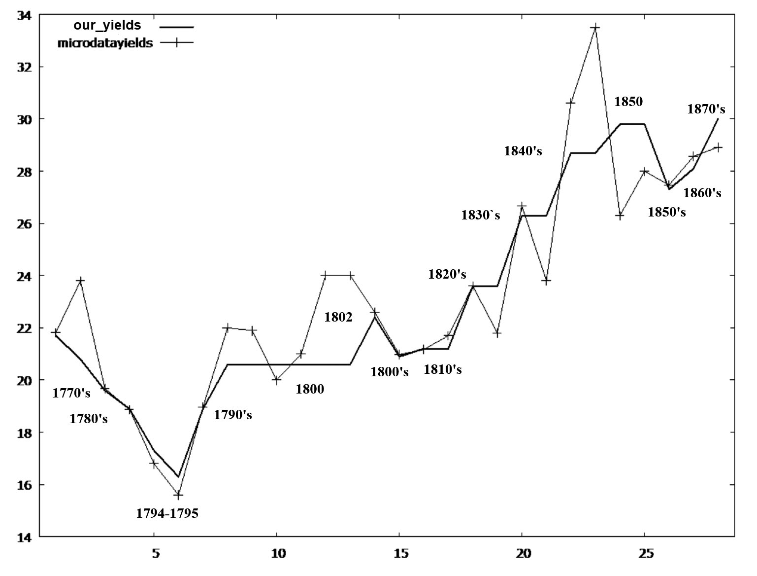
GRAPH 3
Gross yields in bu/acre of our series V of English wheat production,
compared to those resulting from other site-specific sources indicated
in the previous tables, 1760-1870
Source: our own calculation.
The above does not preclude the existence of a structural change during the
second half of the 18th century, through which income elasticity would have gained momentum along with
the growing income per capita. If we try to incorporate this ascending effect
in series I, lengthening it until 1850 with an average income elasticity of 0.6
(that is, close to 0 until the mid-18th century and growing to 1 in the 19th century), we see how the evolution of the wheat output, demand and yields
obtained fit the trends observed by economic historians so far (series V and
VI, Graphs 3 and 5, Table 7). The correlation coefficient between our gross
yield estimations of wheat per acre and those observed in the main sources is
90%, and average deviation between them is only 1%. These results have been
obtained through a logarithmic regression model of the series between 1640 and
1870: we obtain a non-linear equation of Dwheat = P-0,65wheat P0,8agric I0,6, where Dwheat stands for the national demand of wheat in bushels, Pwheat stands for wheat prices, Pagric is the centennial index of agricultural prices and I stands for the British centennial GDP (Broadberry et al., 2015). The addition of the three elasticities is not equal to zero, since we
are not in perfect competition.
However, the accuracy of these results depends to a high degree on two
variables: the wheat cultivated area and the difference between the gross and
net outputs; that is, the resulting quantity after deducting the part allocated
to seeds, personal consumption, payments in kind, animal feeding or losses.
This stands true for the whole period analysed here. The number of acres of
land used in wheat cultivation is unknown, but there is evidence that
demographic pressure, together with prices and income changes, strongly
affected its evolution in the long term. All published researches assume that
from the second half of the 17th century on, the wheat cultivated area grew steadily until soon after the massive
introduction of the American grain imports during the 1870s and 1880s. Robert
Allen (2005) provided the estimates of 1.4 million of acres in 1700, 2.1 in
1750, 2.5 in 1800, and 3.6 in 1850. The statistical series of wheat cropland
surface began in 1867 with 3.37 million acres.
Regarding the difference between net and gross yields per acre, what we can say
on the whole is that this difference must have been between 2 and 2.5. Peter J.
Bowden (1985) provided some site-specific estimates on wheat harvest detraction
of seeds for sowing and animal feeding ranging from 2.25 to 3.37 bushels/acre
between 1670 and 1745. Mark Overton (1984) quoted Bennet (2-2.5 bu/acre) and
King (who estimated a range of seed-yield ratios from 1:4 to 1:8). Anthony
Wrigley (1987) suggested a reference value of 2.5 (quoting Bowden and Slicher
van Bath), plus 1 in other cereals for cattle-feeding. In some passages in
their writings on agriculture, Robert Plot and John Mortimer claimed that
farmers sowed between 2 and 2.5 bu/acre of wheat, or 2 bu/acre in poor soils
and 3 in the most productive, respectively (Plot, 1705: 250; Mortimer, 1712:
95). All of these estimates exclude personal consumption, payments in kind or
simply losses within farms.
Our series can also be compared with the crop estimates provided by English
agricultural historiography. William G. Hoskins (1968: 20-2) described as
deficient those crops from the years 1646, 1657, 1710, and 1711; as bad or very
bad crops those from the years 1647, 1648, 1649, 1658, 1661, 1662, 1673, 1674,
1678, 1692, 1693, 1695, 1696, 1697, 1698, 1708, 1709, 1714, 1727, 1728, and
1729; as “average” crops those from the years 1699, 1700, 1718, 1719, and 1720; and as good crop
years those from 1652, 1653, 1654, 1655, 1665-72, together with the 1680s,
generally good, as well as the periods 1700-07 and 1721-23. Peter Bowden (1985:
56) suggested the existence of bad crops in the second half of the 17th century in the periods 1645-51, 1656-63, 1695-99 and good crops in the periods
1664-72, 1685-91, 1714-24, and 1741-49. Our series fits the period 1640-1750
quite well (Table 8).
GRAPH 4
Long-term evolution of English wheat yields in bu/acre, from 1645 to 1850
Source: our own calculation.
GRAPH 5
Long-term comparison of our estimates of English wheat output and demand in
millions of bushels (series V and VI)
Source: our own calculation.
Table 7
Comparison of different estimates of English wheat yields, 1760-1879
| Years | Our estimates (gross, bu/acre) | Other authors (gross, bu/acre) | Deviation | Authors |
| 1760-69 | 21.7 | 21.82 | 0.5% | Turner et al. (2001) |
| 1770 | 20.8 | 23.80 | 12.6% | Artur Young (John, 1986) |
| 1770-79 | 19.6 | 19.68 | 0.4% | Turner et al. (2001) |
| 1780-89 | 18.9 | 18.88 | -0.1% | Turner et al. (2001) |
| 1794 | 17.3 | 16.8 | -3.0% | Harvest inquiry (John, 1986) |
| 1795 | 16.3 | 15.6 | -4.5% | Harvest inquiry (John, 1986) |
| 1790-99 | 18.9 | 18.97 | 0.4% | Turner et al. (2001) |
| 1800 | 20.6 | 22 | 6.4% | Oxon (Allen, 2005) |
| 1800 | 20.6 | 21.9 | 5.9% | Harvest inquiry (John, 1986) |
| 1800 | 20.6 | 20 | -3.0% | England (Allen, 2005) |
| 1800 | 20.6 | 21 | 1.9% | Hants (Glennie, 1991) |
| 1800 | 20.6 | 24 | 14.2% | Herts (Glennie, 1991) |
| 1800 | 20.6 | 24 | 14.2% | Holderness (1989) |
| 1802 | 22.4 | 22.6 | 0.9% | Crop Ret. (Turner et al., 2001) |
| 1800-09 | 20.9 | 20.98 | 0.4% | Turner et al. (2001) |
| 1810-19 | 21.2 | 21.17 | -0.1% | Turner et al. (2001) |
| 1810-19 | 21.2 | 21.7 | 2.3% | Healy and Jones (1962) |
| 1820-29 | 23.6 | 23.6 | 0.0% | Turner et al. (2001) |
| 1820-29 | 23.6 | 21.8 | -8.3% | Healy and Jones (1962) |
| 1830-39 | 26.3 | 26.67 | 1.4% | Turner et al. (2001) |
| 1830-39 | 26.3 | 23.8 | -10.5% | Healy and Jones (1962) |
| 1840-49 | 28.7 | 30.6 | 6.2% |
Turner et al. (2001) |
| 1840-49 | 28.7 | 33.5 | 14.3% | Healy and Jones (1962) |
| 1850 | 29.8 | 26.3 | -13.3% | Craigie (1883; from Turner et al., 2001) |
| 1850 | 29.8 | 28 | -6.4% | Allen (2005) |
| 1850-59 | 27.3 | 27.47 | 0.6% |
Turner et al. (2001) |
| 1860-69 | 28.1 | 28.57 | 1.6% | Turner et al. (2001) |
| 1870-79 | 30 | 28.92 | -3.7% | Turner et al. (2001) |
| Mean | 23.03 | 23.36 | 1.1% | |
| Median | 21.2 | 22.3 | 0.5% | |
| Minimum | 16.3 | 15.6 | -13.3% | |
| Maximum | 30 | 33.5 | 14.3% | |
| Standard deviation | 4.07 | 4.160 | 0.07 | |
| C.V. | 0.177 | 0.178 | 6.23 | |
Source: our own calculation. The correlation coefficient between the two columns is 0.9.
Table 8
Comparison of the variation of our English series of gross wheat output
with the available chronology of the character of harvests, 1645-1749
| Hoskins | Years | Wheat gross output (bushels) |
| Deficient crops | 1646, 1657, 1710, 1711 | 31,306,518 (-8.8%) |
| Bad and very bad crops | 1647, 1648, 1649, 1658, 1661, 1662, | |
| 1673, 1674, 1678, 1692, 1693, 1695, | 30,330,181 (-11.6%) |
| 1696, 1697, 1698, 1708, 1709, 1714, |
| 1727, 1728, 1729 | |
| Average crops | 1699, 1700, 1718, 1719, 1720 | 34,302,075 |
| Good years | 1652, 1653, 1654, 1655, 1665-72, |
| 1680s generally good, 1700-07 | 35,332,446 (+3%) |
| and 1721-23 | |
| Bowden | Years | Wheat gross output (bushels) |
| Bad crops | 1645-51 | 29,696,256 |
| 1656-63 | 30,491,192 |
| 1695-99 | 29,886,137 |
| Good crops | 1664-72 | 34,251,154 |
| 1685-91 | 35,718,380 | |
| 1714-24 | 34,976,126 |
| 1741-49 | 37,842,623 | |
Source: our own calculation.
This verification can be completed by comparing Table 8 with the sequence of
food riots studied by John Bohstedt (2010), a clear coincidence being observed
with the worst production years. Furthermore, our annual series of wheat
production also allows us to clear up some discrepancies. For example, Hoskins
claimed that 1699 was an average year, whereas Bowden considered it bad. Who
was right? Our results are 29.7 million bushels, a low figure. Therefore, it
would appear that Bowden was closer to reality.
5. CONCLUSIONS
This article presents the first estimation of the English annual series of wheat
production, yields (considering acreage) and demand (adding foreign net trade
balance) for a period for which these data are unknown: 1645-1761. The
methodology applied is based on the price elasticity in England calculated by
Charles Davenant in 1699, anchoring the series on the “usual” average harvest of 1700 and setting a long-term trend based on population and
income growth in a way that allows supply and demand to be integrated by
considering a slow increase in income elasticity from 1750 onwards. The results
match the available estimates on yields and harvests gathered from
site-specific farm accounts and probate inventories from that period, and also
indicate that the starting points used by Broadberry et al. (2015) to build up the agricultural GDP in 1700 are reliable, at least in the
case of wheat.
Through this exercise, Davenant’s Law has been revealed to be much more accurate than just guesswork, probably
because it was based on well-grounded empirical knowledge of British traders at
the time. The series generated fits well with the independent sources available
and confirms both the decreasing trend of price elasticity in the very long
term (Campbell & Ó Gráda, 2011) and historiography on the variability of wheat crops (Hoskins, 1968;
Bowden, 1985; Bohstedt, 2010).
The estimates carried out in the article suggest that income elasticity had
little significant effect on consumption decisions, at least until the mid-18th century, increasing in importance at a later date. If we lengthen the series to
the year when official statistics began in 1884, assuming an income elasticity
of 0.6 for the whole period 1645-1884, the trend fits the available estimates
on yields and output. The series confirms that wheat production and yields
evolved negatively during the second half of the 18th century, and took off dramatically in the 19th century. Accordingly, seen from a production and yields perspective, the
Agricultural Revolution seems to have taken place in two very different
periods, before 1750 and after 1800.
However, many questions remain open. The change in surface area cultivated with
wheat must be better studied. It is necessary to consider possible changes in
the percentage allocated to seeds in more detail, as well as their uses other
than market sale. The new estimates should also be extended to other cereals
until 1884. The reasons behind the structural breakpoint found around 1761 must
also be found, when wheat yields started to fall, total wheat production slowed
down, England became a net importer, prices rocketed, and physical wheat
consumption per head fell, despite bread intake remaining more stable thanks to
substitution among grains.
Acknowledgments
The authors thank to the participants in the first seminars where this article
was presented as early working paper: “Old and New Worlds: The Global Challenges of Rural History”, ISCTEIUL (University Institute of Lisbon, January 2016), and the PhD Seminar
on Economic History at the University of Barcelona (February 2016). Also,
authors thank to the anonymous reviewer of Historia Agraria for his contributions to improve this article. This work has been funded by the
Spanish projects HAR2014-54891-P and HAR2015-69620-C2-1-P, and the
international Partnership Grant SSHRC 895-2011-1020 on “Sustainable Farm Systems: Long-Term Socio-ecological Metabolism in Western
Agriculture” funded by the Social Sciences and Humanities Research Council of Canada.
REFERENCES
Abler, D. (2010). Demand Growth in Developing Countries. OECD Food, Agriculture and Fisheries Papers, (29).
Allen, R. C. (1988). The Growth of Labor Productivity in Early Modern English Agriculture. Explorations in Economic History, 25 (2), 117-46.
Allen, R. C. (1989). Enclosure, Farming Methods and the Growth of Productivity in the South
Midlands. In G. Grantham & C. S. Leonard (Eds.), Agrarian Organization in the Century of Industrialization: Europe, Russia, and
North America (pp. 69-88). Greenwich: Jai Pr. (Research in Economic History, suppl. 5).
Allen, R. C. (1991). The Two English Agricultural Revolutions, 1450-1850. In B. S. M. Campbell & M. Overton (Eds.), Land, Labour and Livestock: Historical Studies in European Agricultural
Productivity (pp. 236-54). Manchester: Manchester University Press.
Allen, R. C. (1999). Tracking the Agricultural Revolution in England. Economic History Review, (52), 209-35.
Allen, R. C. (2005). English and Welsh Agriculture, 1300-1850: Outputs, Inputs and Income. Oxford University Working Papers.
Allen, R. C. (2007). Pessimism Preserved: Real Wages in the British Industrial Revolution. Oxford University Working Papers.
Allen, R. C. (2008). The Nitrogen Hypothesis and the English Agricultural Revolution: A
Biological Analysis. The Journal of Economic History, 68 (1), 182-210.
Allen, R. C. (2009). The British Industrial Revolution in Global Perspective. Cambridge: Cambridge University Press.
Appleby, A. B. (1979). Grain Prices and Subsistence Crises in England and France, 1590-1740. The Journal of Economic History, 39, (4), 865-87.
Barquín, R. (2005). The Elasticity of Demand for Wheat in the 14th to 18th Centuries. Revista de Historia Económica-Journal of Iberian and Latin American Economic History, 23 (2), 241-68.
Bohstedt, J. (2010). The Politics of Provisions: Food Riots, Moral Economy and Market Transition in
England, 1550-1850. Farnham: Ashgate.
Bowden, P. (1985). Agricultural Prices, Wages, Farm Profits, and Rents. In J. Thirsk (Ed.), The Agrarian History of England and Wales. 5: 1640-1750. Part 2: Agrarian Change (pp. 1-117). Cambridge: Cambridge University Press.
Broadberry, S., Campbell, B. M. S., Klein, A., Overton, M. & Van Leeuwen, B. (2015). British Economic Growth, 1270-1870. Cambridge: Cambridge University Press.
Brunt, L. (2004). Nature or Nurture? Explaining English Wheat Yields in the Industrial
Revolution, c. 1770. The Journal of Economic History, 64 (1), 193-225.
Brunt, L. (2015). Weather Shocks and English Wheat Yields, 1690-1871. Explorations in Economic History, (57), 50-58.
Caird, J. (1852). English Agriculture. London: Cassell.
Campbell, B. M. S. & Ó Gráda, C. (2011). Harvest Shortfalls, Grain Prices, and Famines in Preindustrial England.
The Journal of Economic History, 71 (4), 859-86.
Chartres, J. A. (1985). The Marketing of Agricultural Produce. In J. Thirsk (Ed.), The Agrarian History of England and Wales. 5: 1640-1750. Part 2: Agrarian Change (pp. 406-502). Cambridge: Cambridge University Press.
Chartres, J. A. (1995). Market Integration and Agricultural Output in Seventeenth-, Eighteenth-,
and early Nineteenth-Century England. The Agricultural History Review, 43 (2), 117-38.
Clark, G. (2002). The Agricultural Revolution and the Industrial Revolution: England,
1500-1912. University of California Working Paper.
Clark, G. (2004). The Price History of English Agriculture, 1209-1914. Research in Economic History, (22), 41-124.
Clark, G. (2005). The Condition of the Working-Class in England, 1209-2004. Journal of Political Economy, 113 (6), 1307-40.
Clark, G. (2007). The Long March of History: Farm Wages, Population and Economic Growth,
England 1209-1869. Economic History Review, 60 (1), 97-135.
Clark, G., Cummings, J. & Smith, B. (2010). The Surprising Wealth of Pre-industrial England. SSRN Working Paper.
Collins, E. J. T. (1975). Dietary Change and Cereal Consumption in Britain in the Nineteenth
Century. The Agricultural History Review, 23 (2), 97-115.
Comber, W. T. (1808). An Inquiry into the State of National Subsistence as connected with the Progress
of Wealth and Population. London: T. Cadell & W. Davis.
Crafts, N. F. R. (1980). Income Elasticities of Demand and the Release of Labor by Agriculture
during the British Industrial Revolution: A Further Appraisal. Journal of European Economic History, (9), 153-68.
Davenant, C. (1771[1699]). An Essay upon the Probable Methods of Making a People Gainers in
the Balance of Trade. In C. Whitworth (Ed.), The Political and Commercial Works of Charles Davenant. London: R. Horsfield.
Davies, D. (1795). The Case of Labourers in Husbandry. London: C. G. & J. Robinson.
Deane, P. & Cole, W. A. (1967). British Economic Growth, 1688-1959, Trends and Structure. 2nd ed. Cambridge: Cambridge University Press.
Eden, F. M. (1797). The State of the Poor. London: Cass.
Endres, A. M. (1987). The King-Davenant “Law” in Classical Economics. History of Political Economy, 19 (4), 621-38.
Fogel, R. W. (2004). The Escape from Hunger and Premature Death, 1700-2100: Europe, America, and the
Third World. Cambridge: Cambridge University Press.
Glennie, P. (1991). Measuring Crop Yields in Early Modern England. In B. M. S. Campbell & M. Overton (Eds.), Land, Labour and Livestock: Historical Studies in European Agricultural
Productivity (pp. 255-83). Manchester: Manchester University Press.
Healy, M. J. R. & Jones, E. L. (1962). Wheat Yields in England, 1815-59. Journal of the Royal Statistical Society. Series A (General), 125 (4), 574-79.
Hipkin, S. (2012). The Coastal Metropolitan Corn Trade in Later Seventeenth Century
England. The Economic History Review, 65 (1), 220-55.
Holderness, B. A. (1989). Prices, Productivity, and Output. In G. E. Mingay (Ed.), The Agrarian History of England and Wales. 6: 1750-1850 (pp. 1-118). Cambridge: Cambridge University Press.
Hoskins, W. G. (1968). Harvest Fluctuations and English Economic History, 1620-1759. The Agricultural History Review, 16 (1), 15-31.
Hoyle, R. W. (2013). Why was there no Crisis in England in the 1690’s? In R. W. Hoyle (Ed.), The Farmer in England, 1650-1980 (pp. 69-100). London: Routledge.
Hutchison, T. W. (1988). Before Adam Smith: The Emergence of Political Economy, 1662-1776. Oxford: Blackwell.
John, A. H. (1986). Statistical Appendix. In G. E. Mingay (Ed.), The Agrarian History of England and Wales. 6: 1750-1850 (pp. 972-1155). Cambridge: Cambridge University Press.
Jones, E. L. (1965). Agriculture and Economic Growth in England, 1660-1750: Agricultural
Change. The Journal of Economic History, 25 (1), 1-18.
Kain, R. J. P. & Prince, H. C. (2006). The Tithe Surveys of England and Wales. Cambridge: Cambridge University Press.
Kelly, M. & Ó Gráda, C. (2013). Numerare Est Errare: Agricultural Output and Food Supply in England Before and During the
Industrial Revolution. The Journal of Economic History, 73 (4), 1132-163.
Kerridge, E. (1967). The Agrarian Revolution. London: George Allen & Unwin.
Lawes, J. B. & Gilbert, J. H. (1893). Home produce, Imports, Consumption and Price of Wheat over 40 Harvest-Years,
1852-3 to 1891-2. London: Spottiswoode.
Mitchell, B. R. (1988). British Historical Statistics. Cambridge: Cambridge University Press.
Mortimer, J. (1712). The Whole Art of Husbandry: Or, the Way of Managing and Improving of Land.
Being a Full Collection of what Hath Been Writ, Either by Ancient Or Modern
Authors:... As Also an Account of the Particular Sorts of Husbandry Used in
Several Counties;... To which is Added, the Country-man’s Kalendar. London: R. Robinson.
Neild, W. (1841). Comparative Statement of the Income and Expenditure of Certain Families
of the Working Classes in Manchester and Duckenfield, in the Years 1836 and
1841. Journal of the Statistical Society of London, 4 (4), 320-34.
Nielsen, M., Smit, J. & Guillén, J. (2012). Price Effects of Changing Quantities Supplied at the Integrated European
Fish Market. Marine Resource Economics, 27 (2), 165-80.
Ormrod. D. (1985). English Grain Exports and the Structure of Agrarian Capitalism, 1700-1760. Hull: Hull University Press.
Overton, M. (1979). Estimating Crop Yields from Probate Inventories: An Example from East
Anglia, 1585-1735. The Journal of Economic History, 39 (2), 363-78.
Overton, M. (1984). Agricultural Productivity in Eighteenth-Century England: Some Further
Speculations. The Economic History Review, 37 (2), 252-57.
Overton, M. (1991). The Determinants of Crop Yields in Early Modern England. In B. M. S. Campbell & M. Overton (Eds.), Land, Labour and Livestock: Historical Studies in European Agricultural
Productivity. Manchester: Manchester University Press.
Overton, M. (1996a). Re-Establishing the English Agricultural Revolution. The Agricultural History Review, 44 (1), 1-20.
Overton, M. (1996b). Agricultural Revolution in England: The Transformation of the Agrarian Economy,
1500-1850. Cambridge: Cambridge University Press.
Parenti, G. (1942). Prezzi e mercato del grano a Siena, 1546-1765. Firenze: C. Cya.
Persson, K. G. (1999). Grain Markets in Europe, 1500-1900: Integration and Deregulation. Cambridge: Cambridge University Press.
Petersen, C. (1995). Bread and the British Economy, c 1770-1870. Aldershot: Scholar Press.
Petty, W. (1927 [1687]). The Petty Papers: Some Unpublished Writings of Sir William Petty. London: Constable.
Plot, R. (1705 [1676]). The Natural History of Oxford-Shire, Being an Essay towards the Natural History
of England. London: Leon Lischfield, for Charles Brome and J. Nicholson.
Rogers, J. E. T. (1877). A History of Agriculture and Prices in England. 6: 1583-1702. Oxford: Clarendon.
Simonin, J. P. (1996). Des premiers énoncés de la loi de King à sa remise en cause: Essais de mesures ou fictions théoriques. Histoire & Mesure, 11 (3-4), 213-54.
Slicher van Bath, B. H. (1963). The Agrarian History of Western Europe: A. D. 500-1850. London: Edward Arnold.
Tello, E., Martínez, J. L., Jover, G., Olarieta, J. R., García Ruiz, R., González de Molina, M., Badia, M., Winiwarter, V. & Koepke, N. (2017). The Onset of the English Agricultural Revolution: Climate Factors and
Soil Nutrients. The Journal of Interdisciplinary History, 47 (4), 445-74.
Theobald, J. (2002). Agricultural Productivity in Woodland High Suffolk, 1600-1850. The Agricultural History Review, 50 (1), 1-24.
Tooke, T. & Newmarch, W. (1838). A History of Prices, and of the State of the Circulation, from 1793 to 1837. London: Longman, Orme, Brown, Green, and Longmans.
Turner, M. (1982). Agricultural Productivity in England in the Eighteenth Century: Evidence
from Crop Yields. The Economic History Review, 35 (4), 489-510.
Turner, M. (1986). English Open Fields and Enclosures: Retardation or Productivity
Improvements. The Journal of Economic History, 46 (3), 669-92.
Turner, M. E., Becket, J. V. & Afton, B. (1997). Agricultural Rent in England, 1690-1914. Cambridge: Cambridge University Press.
Turner, M. E., Becket, J. V. & Afton, B. (2001). Farm Production in England, 1700-1914. Oxford: Oxford University Press.
Uebele, M., Grünebaum, T. & Kopsidis, M. (2013). King’s Law and Food Storage in Saxony, c. 1790-1830. Center for Quantitative Economics Working Papers, (26).
Wrigley, E. A. (1987). People, Cities and Wealth. Oxford: Blackwell.
Wrigley, E. A. & Schofield, R. S. (1981). The Population History of England, 1541-1871: A Reconstruction. Cambridge: Cambridge University Press.
Yelling, J. A. (1970). Probate Inventories and the Geography of Livestock Farming: A Study of
East Worcestershire, 1540-1750. Transactions of the Institute of British Geographers, (51), 111-26.
Yelling, J. A. (1973). Changes in Crop Production in East Worcestershire 1540-1867. Agricultural. History Review, 21 (1), 18-34.
APPENDIX
| WHEAT GROSS OUTPUT |
YEAR | (BROAD_POP, SERIES I) |
| Million bushels |
| 1640 | 34.5 |
| 1641 | 32.2 |
| 1642 | 33.5 |
| 1643 | 32.9 |
| 1644 | 33.5 |
| 1645 | 33.7 |
| 1646 | 32.3 |
| 1647 | 28.8 |
| 1648 | 27.3 |
| 1649 | 28.1 |
| 1650 | 28.5 |
| 1651 | 29.3 |
| 1652 | 31.6 |
| 1653 | 35.3 |
| 1654 | 38.9 |
| 1655 | 39.6 |
| 1656 | 33.6 |
| 1657 | 32.8 |
| 1658 | 30.0 |
| 1659 | 29.3 |
| 1660 | 30.2 |
| 1661 | 28.9 |
| 1662 | 27.9 |
| 1663 | 31.1 |
| 1664 | 31.6 |
| 1665 | 33.2 |
| 1666 | 36.1 |
| 1667 | 36.9 |
| 1668 | 36.2 |
| 1669 | 32.6 |
| 1670 | 33.9 |
| 1671 | 33.5 |
| 1672 | 34.3 |
| 1673 | 33.3 |
| 1674 | 29.2 |
| 1675 | 30.5 |
| 1676 | 35.5 |
| 1677 | 34.6 |
| 1678 | 31.6 |
| 1679 | 31.0 |
| 1680 | 33.6 |
| 1681 | 32.3 |
| 1682 | 32.7 |
| 1683 | 33.1 |
| 1684 | 32.6 |
| 1685 | 32.2 |
| 1686 | 35.3 |
| 1687 | 34.9 |
| 1688 | 37.2 |
| 1689 | 37.8 |
| 1690 | 35.9 |
| 1691 | 36.7 |
| 1692 | 32.1 |
| 1693 | 29.9 |
| 1694 | 30.1 |
| 1695 | 32.5 |
| 1696 | 30.3 |
| 1697 | 29.1 |
| 1698 | 28.0 |
| 1699 | 29.7 |
| 1700 | 32.9 |
| 1701 | 35.9 |
| 1702 | 38.1 |
| 1703 | 38.5 |
| 1704 | 34.9 |
| 1705 | 37.5 |
| 1706 | 38.6 |
| 1707 | 38.2 |
| 1708 | 34.5 |
| 1709 | 28.5 |
| 1710 | 28.1 |
| 1711 | 32.0 |
| 1712 | 33.8 |
| 1713 | 33.0 |
| 1714 | 31.1 |
| 1715 | 35.3 |
| 1716 | 33.2 |
| 1717 | 33.9 |
| 1718 | 35.7 |
| 1719 | 37.2 |
| 1720 | 34.6 |
| 1721 | 35.5 |
| 1722 | 36.4 |
| 1723 | 35.6 |
| 1724 | 36.2 |
| 1725 | 33.8 |
| 1726 | 32.5 |
| 1727 | 33.9 |
| 1728 | 30.3 |
| 1729 | 31.9 |
| 1730 | 35.7 |
| 1731 | 37.5 |
| 1732 | 40.8 |
| 1733 | 39.0 |
| 1734 | 36.0 |
| 1735 | 33.9 |
| 1736 | 34.5 |
| 1737 | 36.7 |
| 1738 | 37.6 |
| 1739 | 36.3 |
| 1740 | 32.3 |
| 1741 | 32.1 |
| 1742 | 37.9 |
| 1743 | 40.9 |
| 1744 | 41.6 |
| 1745 | 39.8 |
| 1746 | 36.7 |
| 1747 | 37.6 |
| 1748 | 36.8 |
| 1749 | 37.1 |
| 1750 | 37.5 |
| 1751 | 36.0 |
| 1752 | 34.5 |
| 1753 | 34.7 |
| 1754 | 36.8 |
| 1755 | 38.2 |
| 1756 | 35.2 |
| 1757 | 30.9 |
| 1758 | 33.6 |
| 1759 | 37.6 |
| 1760 | 39.0 |
| 1761 | 39.6 |